![]() (1)
(1)
Improved Intra-Species Collision Models for PIC Simulations
Michael E. Jones, D. S. Lemons, and D. Winske,
Plasma Physics Applications Group,
Applied Theoretical & Computational Physics Division,
Los Alamos National Laboratory
Los Alamos, NM 87545
In recent years, we have investigated methods to improve the effectiveness of modeling collisional processes in particle-in-cell codes. Through the use of generalized collision models, plasma dynamics can be followed both in the regime of nearly collisionless plasmas as well as in the hydrodynamic limit of collisional plasmas. We have developed a collision-field method to treat both the case of collisions between unlike plasma species ("inter-species collisions"), through the use of a deterministic, grid-based force, and between particles of the same species ("intra-species collisions"), through the use of a Langevin equation (Jones et al., 1996a). While the approach used for inter-species collisions is "noise-free" in that the collision experienced by a particle does not require any random numbers, such random numbers are used for intra-species collisions. This gives rise to a stochastic cooling effect inherent in the Langevin approach (Lemons et al., 1995). In this paper, we concentrate on intra-species collisions and describe how the accuracy of the model can be improved by appropriate corrections to velocity and spatial moments.
The usual approach to model Coulomb collisions in a particle-in-cell (PIC) code is to pair up particles and scatter each pair elastically in every computational cell each time step (Takizuka and Abe, 1997). This method assures that energy and momentum are locally conserved. However, there is some arbitrariness in pairing the particles, and the time step must be small enough so that each collision is resolved. And this method is computationally intensive, although recent work has shown that the process can be vectorized efficiently (Wang et al., 1996).
An alternative approach, which we refer to as the collision-field method (Jones et al., 1996a), is based on the concept of particles being scattered by a collision force defined locally and instantaneously throughout the simulation space-time. The basic physics of the collisional interaction is included through a set of collision rates, which themselves are scalar functions of local fluid quantities. In our implementation, the collision rates, like electromagnetic field quantities, are accumulated on the grid of the simulation and updated each time step. Collisions between plasma particles of the same kind, i.e., intra-species collisions, impulsively and randomly exchange energy and momentum. We achieve this by advancing particle velocities with exact solutions to a three parameter linear Langevin equation, i.e., as an Ornstein-Uhlenbeck (O-U) stochastic process (Gillespie, 1992). The three parameters are: a self collision rate
n, and a mass-weighted velocity mean m, and standard deviation (i.e., temperature). The latter are chosen to ensure that, on average, the species conserves its total energy and momentum. Although other processes can be conceived which more fully implement the nonlinear physics of small angle Coulomb collisions, an O-U process is the simplest one having the above desirable properties. For this reason, it is particularly well suited both for computations and for exact analysis.We discuss improved methods to treat intra-species collisions. We show that by linearly transforming particle velocity moments each time step, we can conserve momentum and energy exactly, in addition to stochastically scattering particle velocities toward a Maxwellian distribution with the Langevin pusher. Moreover, we demonstrate that some further improvements can be achieved by adjusting the spatial moments of the particles to recover the correct spatial diffusion. It should be noted that, while these collision methods are being applied to model Coulomb collisions in the electromagnetic particle code ISIS, which has been used to study plasma interpenetration and coupling through collisions (Jones et al., 1996b), the basic techniques and the modifications discussed here can be applied to other codes that use Monte Carlo methods as well.
For a system of n particles, the time differenced equation for the velocity advance based on the Langevin equation is (Lemons et al., 1995)
![]() (1)
(1)
where
n is the collision frequency, m is the mean velocity, sv is the thermal velocity, N(0,1) is a random number drawn from a normal distribution with zero mean and variance of one, and subscript i refers to particle number, i=1,2...n. When n, m, and sv are independent of v and t, (1) defines the Ornstein-Uhlenbeck (U-O) process, which conserves energy and momentum.Equation (1) can be solved exactly to give, in difference form
![]() (2)
(2)
where superscript n refers to the time index, and
D t is the time step (with t = n D t). For small n D t, (2) evidently reduces to (1), while for n D t large, each particle has velocity m, and the particle distribution has the appropriate temperature based on sv.
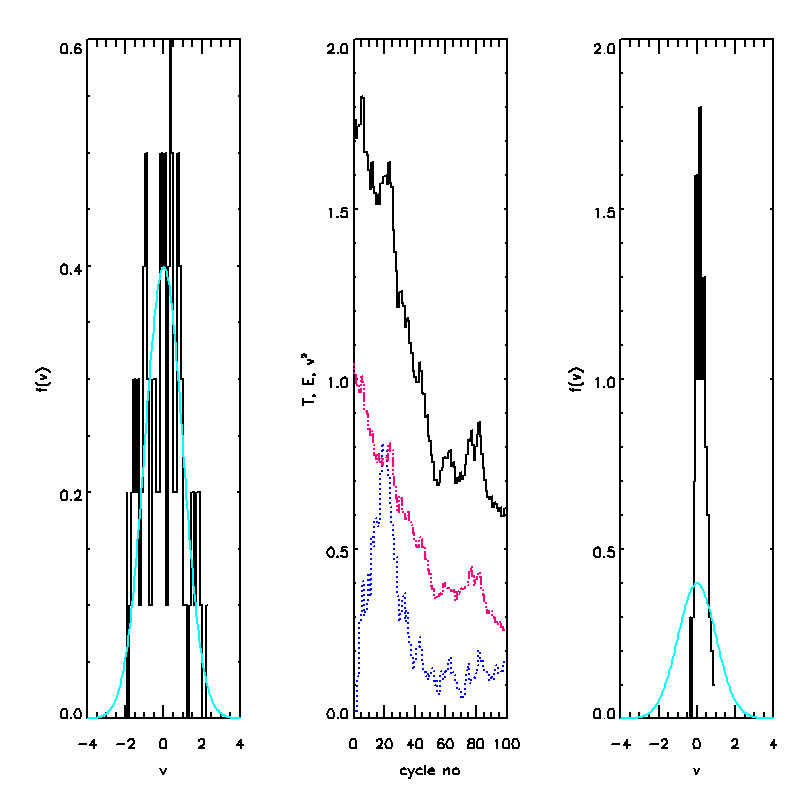
 An example
of the use of Eq. (2) in the interaction of n =100 self-colliding particles is shown in
Figure 1. Plotted in the left panel as a histogram is the initial distribution of the n
particles, with random velocities chosen so that the mean velocity is zero and the
temperature is unity. The superimposed solid curve is the corresponding Maxwellian
distribution. The raggedness of the initial distribution emphasizes the underlying
difficulty in particle codes of representing the velocity distribution with a relatively
small number of particles in each computational cell. The system is then allowed to evolve
in time, by repeated applications of (2). The middle panel of Figure 1 shows time
histories of the mean velocity, the temperature, and the total energy of the system over
100 time steps. While, as expected, fluctuations of the average quantities do occur,
somewhat surprising is the fact that these quantities have a net shift in one direction.
In particular, there is a systematic reduction of the temperature, as well as an increase
of the mean velocity and total energy . This is shown more clearly in the right panel of
Figure 1, where the particle distribution at t=100 is displayed. In spite of the noisiness
of the distribution, the reduction of the temperature and the change in the mean velocity
are clearly evident.
Figure 1. Distribution based on 100 randomly distributed particles at t=0 (left) and after 100 time steps (right) using Eq. (2); time histories of mean velocity (lower curve), temperature(middle curve), and total energy (upper curve) (center).
While only one time sequence has been shown, the tendency for the distribution subject to an O-U process to cool is a well-known effect in stochastic processes (Gillespie, 1992; Lemons et al., 1995). It can be shown using appropriate mathematical techniques that the cooling is exponential in time, exp(-
gt), with g ~ n/n. Hence, for very large particle numbers, the cooling time is much longer than the relaxation time, ~n-1. However, in particle simulations, where the number of particles per cell (n) can be as small as 10, the effect can be significant.Given the inherent simplicity, elegance, and accuracy of the Langevin approach, as well as this embedded numerical instability, we next turn to two ways to improve the model that are effective in the limiting case of interest to us here: namely, relatively large collision frequency,
n D t > 1, and small numbers of particles, n < 1000.The first remedy, and one that we have found is completely satisfactory (Lemons et al., 1995), is to linearly transform the velocities
 (3)
(3)
where the primes refer to quantities that have just been advanced, and
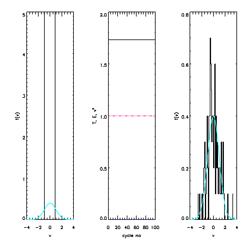
m and sv are the fixed values of the mean velocity and thermal speed. Figure 2, in the same format as Figure 1, shows the effect of applying (3) along with (2) each time cycle. Again, the initial distribution of 100 particles is shown in the left panel, and the distribution of these particles again after 100 time steps is displayed in the right panel. While the distribution itself changes, due to the use of different random numbers, the mean velocity and temperature remain constant. This is further demonstrated by the time histories in the middle panel, which, by construction, remain constant.
Figure 2. Same as Figure 1, but applying the velocity moment correction (3) each time step.
A second, more subtle correction is to modify the positions of the particle so that both the freestreaming (i.e., collisionless) and the diffusion (i.e., strongly collisional) limits are reproduced. The difficulty arises due to the fact that in the highly collisional limit,
nD t >>1, Eq. (2) reduces to![]() (4)
(4)
but
![]() (5)
(5)
In other words, the particles' new positions are a result of many random motions that occur in the time interval
D t, which cannot simply be described in terms of moving each particle with its new velocity (which contains both a directed and a random component). Instead, we correct the position of each particle after each time step in order to reproduce the correct ensemble-averaged spatial diffusion required by the O-U process.In this case, the ensemble-averaged (denoted by an overhead bar) particle position is
![]() (6)
(6)
while individual particle positions are distributed normally with respect to this mean, with a variance,
sx2. The variance is obtained from an appropriate temporal integration of Eq. (2), i.e., (7)
(7)
In practice this means that like the particle velocities , the positions are renormalized each time step so that the average position and the spatial variance are preserved.
Note that in the collisionless limit,
n D t << 1, and in the absence of correlations between the cell averaged particle position and velocity, (7) reduces to![]() (8)
(8)
i.e., the spatial spread is roughly the thermal speed times the time step. In the opposite limit,
nD t >> 1, when the mean free path (l) is resolved, namely when the cell size Dx < l,![]() (9)
(9)
Thus, the spatial spread in this case is proportional to
D t 1/2, consistent with the diffusion limit.In general, the use of "moment corrections" for particle codes appears to be a promising means of reducing noise due to finite particle populations. Other possible corrections will be discussed.
Gillespie, D. T., Markov Processes: An Introduction for Physical Scientists, (Academic Press, San Diego, 1992), pp.111-116.
Jones, M. E., Lemons, D. S., Mason, R. J., Thomas, V. A., and Winske, D., J. Comput. Phys., 123(1), 169-181 (1996a).
Jones, M. E., Winske, D., Goldman, S. R., Kopp, R. A., et al., Phys. Plasmas, 3(3), 1096-1108 (1996b).
Lemons, D. S., Lackman, J., Jones, M. E., and Winske, D., Phys. Res. E, 52(6), 6855-6861 (1995).
Takizuka, T. and Abe, H., J. Comput. Phys. 25(2) 205-219 (1977).
Wang, W. X., Okamoto, M., Nakajima, N., and Murakami, S., J. Comput. Phys., 128(1), 209-222 (1996).