Free Matlab Source Codes for the Generalized Proximal Smoothing (GPS) algorithm
I. Overview
We report the development of the generalized proximal smoothing (GPS) algorithm for phase retrieval of noisy data. GPS is an optimization-based algorithm, in which we relax both the Fourier magnitudes and support constraint. We relax the support constraint by incorporating the Moreau-Yosida regularization and heat kernel smoothing, and derive the associated proximal mapping. We also relax the magnitude constraint into a least squares fidelity term, whose proximal mapping is available as well. GPS alternatively iterates between the two proximal mappings in primal and dual spaces, respectively.
[see M. Pham, P. Yin, A. Rana, S. Osher, J. Miao, "Generalized proximal smoothing (GPS) for phase retrieval," Opt. Express 27, 2792-2808 (2019). in detail].
II. Algorithms
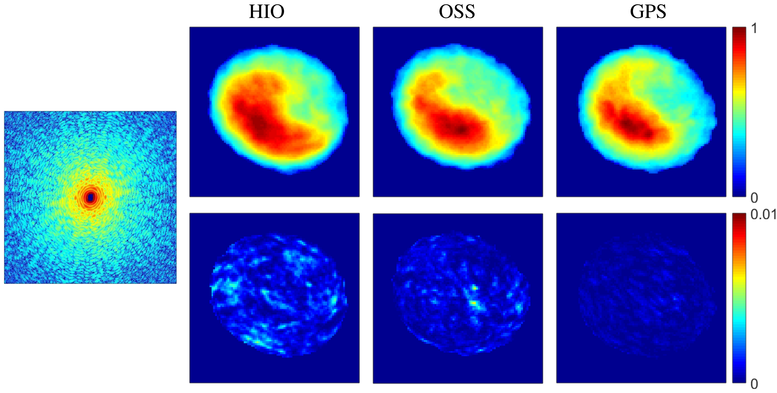
III. Experiments : a. Vesicle model
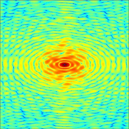
In the sample data used for this simulation, Poisson noise is added to the diffraction intensity with Noise Level at 5%
We record the histogram of the 100 independent runs and the convergence curves of these algorithms
b. S. pombe yeast spore
c. Colloidal gold particles
IV. The Matlab Source Codes of the GPS Algorithm
For all above tests, we provide the codes of a single reconstruction. Users feel free to modify the code to reproduce the full results of our paper, such as the mean, variance, histogram, convergence curve, and comparisons with other methods.
If you use these codes for your publications and/or presentations, we request you cite our paper: M. Pham, P. Yin, A. Rana, S. Osher, J. Miao, "Generalized proximal smoothing (GPS) for phase retrieval" Opt. Express 27, 2792-2808 (2019). For any further questions, comments and/or suggestions, please contact Minh H. Pham (minhrose@ucla.edu).
The idea of phase retrieval is using alternating projection to refine the reconstruction in which the refined object is projected on the magnitude constraint and the support constraint. We replace the alternating projections by generalized proximal smoothing and incorporate the use of dual variable
\begin{align}
1. \quad & z^{k+1} = prox_{t g_ \sigma} ( z^k - t \mathcal{F} y^k ) \\
2. \quad & y^{k+1} = prox_{s f^*_G} \big(y^k + s \mathcal{F}^{-1} (2 z^{k+1} - z^k) \big)
\end{align}
where the proximal is defined to be the backward Euler equation:
\begin{align}
prox_{tf}(x) = \arg \min_y \Big\{ f(y) + \frac{1}{2t} \| y -x \|^2 \Big\} = y \quad \text{where } y \text{ solves the eqn.} \quad y = x - t \nabla f(y)
\end{align}
\( g_{\sigma} (z) = \) \( 1 \over 2 \sigma \) \( \| |z| - b \|^2 \) is the fidelity term to measure the difference between an arbitrary signal \(z\) and the diffraction pattern measurement \(b \).
\( f_{G} (u) = inf_v \{ f(v) + 0.5 \|v-u \|^2_{G^{-1}} \} \) is the proximal with generalized norm \( \| \cdot \|_{G^{-1}} \| \). In addition, \( f_G^*(y) := sup \{ \langle u,y \rangle - f(u)\} \) is the function conjugate of \( f_G \). Thanks to the Moreau-Yosida decomposition, the above conjugate function can be decomposed as below:
$$ f_G^* (y) = f^*(y) + \frac{1}{2} \| y \|^2_{G} $$
\(f(u)\) is the indicator function to the support \( S \) and \( \mathcal{S} := \{ u: u=0 \text{ in } S \} \) is the set of u that satisfies thet support constraint.
So \( f(u) = 0 \) if \( u \in \mathcal{S} \), and equals infinity otherwise.
By definition, we can compute the conjugate to \(f\) as follow: For real and positive object, \(f^*(y) = 0 \) if \( Re(y) \le 0 \) on \( S \), and equals infinity otherwise.
We call \(\mathcal{S}^*\) the corresponding dual set that satifies the dual constraint.
The projection on \( \mathcal{S}^* \) will be computed as follows:
$$
proj_{\mathcal{S}^*} (y)_i =
\begin{cases}
Re(y_i)^- + i \cdot Im(y_i) & \text{if } i \in S \\
y_i & \text{otherwise}
\end{cases}
$$
Both proximals (1) and (2) have exact solution as follow. The first proximal is the relaxation of the projection on the magnitude constraint
$$
prox_{t g_{\sigma}} (z) = \frac{t}{t + \sigma} b \cdot \exp ( i \cdot \arg(z) ) + \frac{\sigma}{t+\sigma} z
$$
The second proximal can be proceeded as follows:
Case 1: Gaussian smoothing on the real space.
The proximal is approximated by two steps: projection on the dual set \(\mathcal{S}^* \) followed by Gaussian smoothing
$$
y^{k+1} = \mathcal{G}_{\gamma} * proj_{\mathcal{S}^*} \big( y^k + s\mathcal{F}^{-1} ( 2 z^{k+1} - z^k ) \big)
$$
Case 2: Gaussian smoothing on the Fourier space. The convolution is replaced by the multiplication
$$
y^{k+1} = \mathcal{G}_{\gamma} \cdot proj_{\mathcal{S}^*} \big( y^k + s\mathcal{F}^{-1} ( 2 z^{k+1} - z^k ) \big)
$$
To search for global minimums, GPS will run with 10 different Gaussian kernel in the decreasing other of variances. The solution with smallest relative error from previous stage will passed on as the initial input to the next stage. Each stage will run for 100 iterations; hence, the total of number of iterations is 1000.
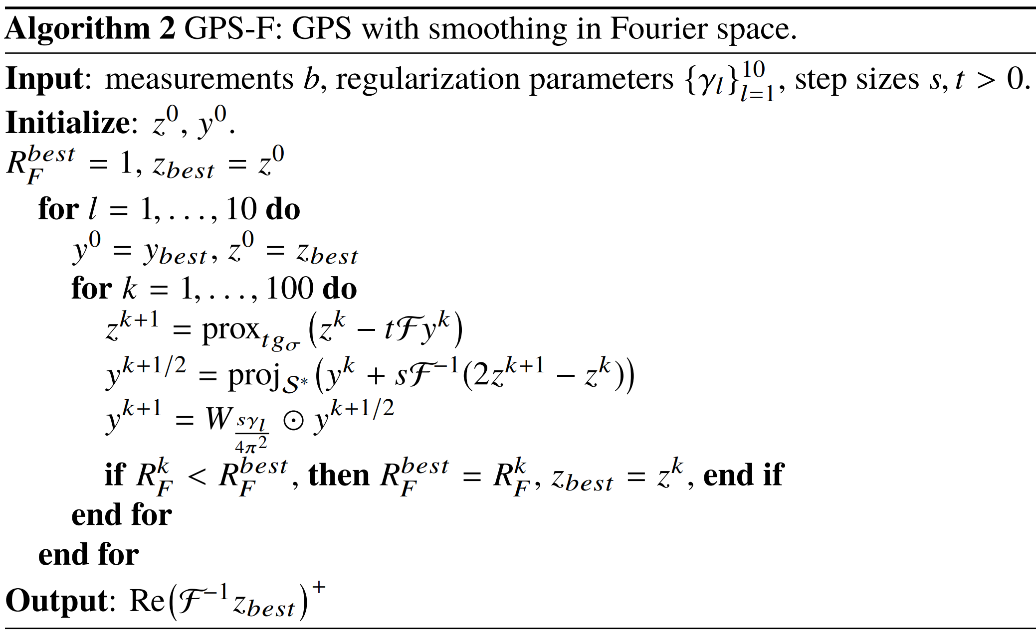
The two algorithms are summarized as bellow: For the smoothing on the real domain, we have GPS-R algorithm
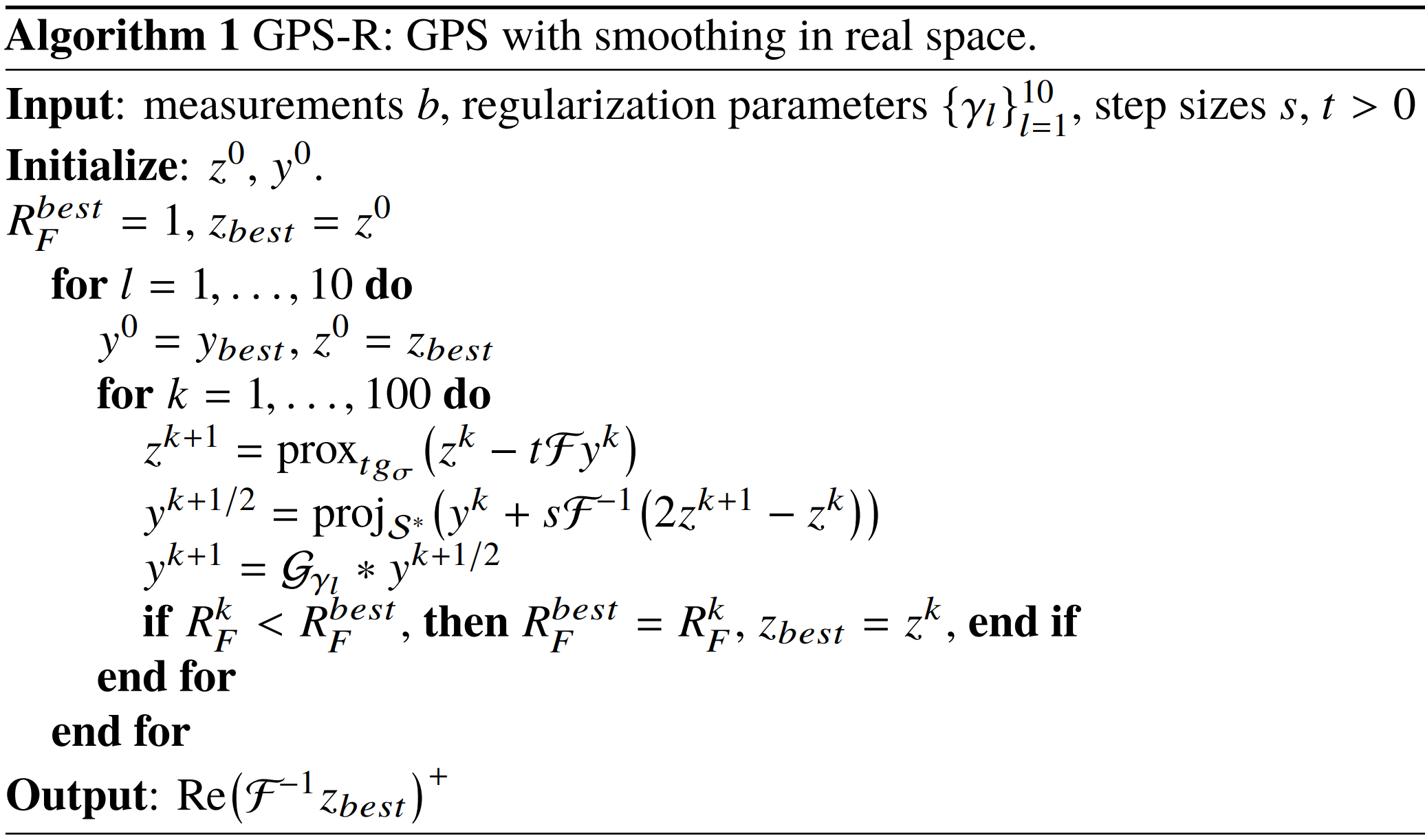
For the smoothing on the frequency space, we have GPS-F algorithm:
We run 100 independent runs with different initialization, then choose the top five reconstructions with smallest relative errors to compute the mean and the variance. The results are compared with HIO and oversampling smoothness OSS
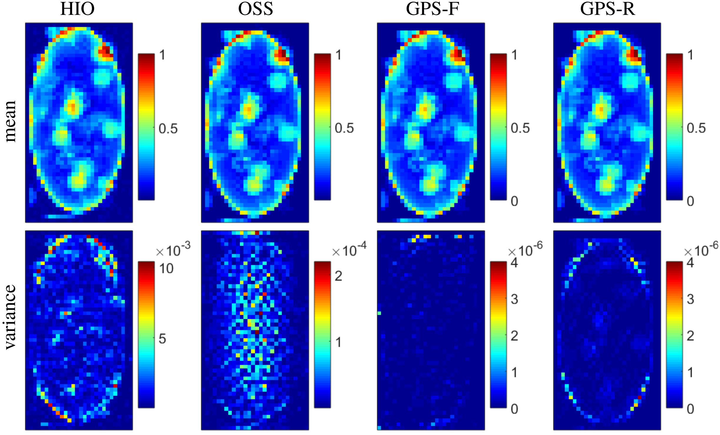
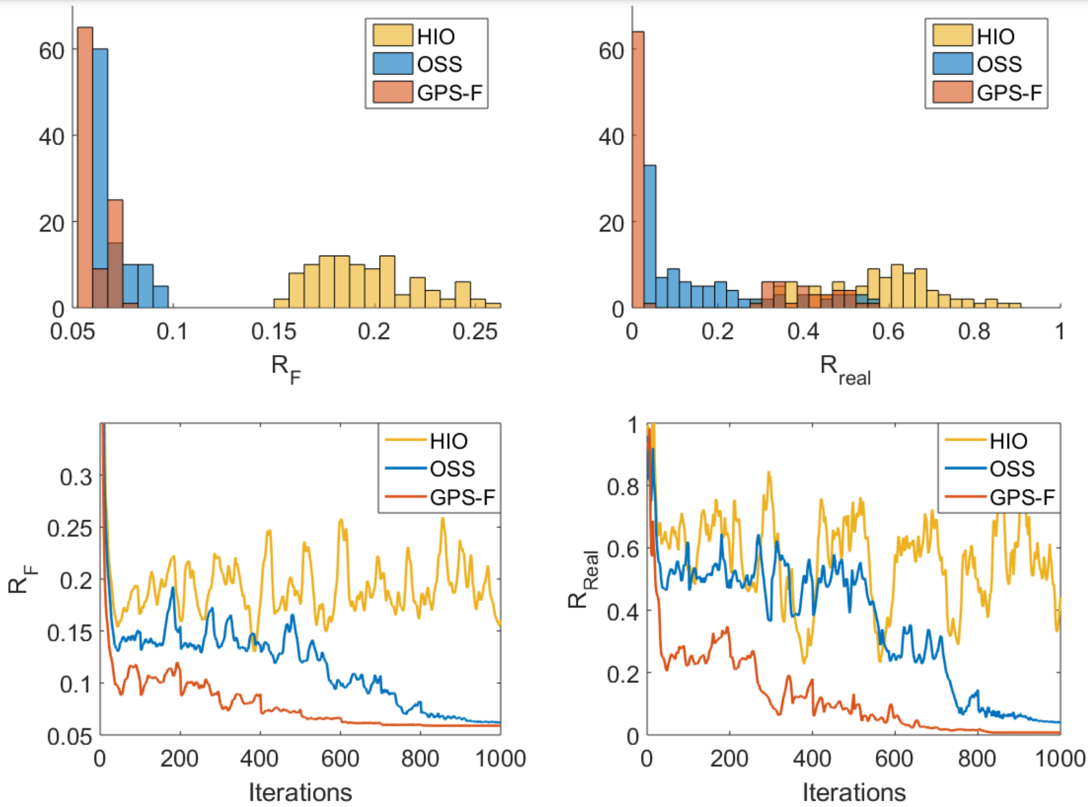
GPS is shown to have higher performance and consitency than other methods. Furthermore, the convergence is smoother with less oscilation and more robust to noise.
Diffraction pattern of S. Pombe yeast spore was obtained from an experiment using beamline BL29 at SPring-8. We do 500 independent, record the reconstruction with five smallest relative errors, then compute the mean and the variance as before
For this reconstruction, we use a loose support with a square shape. Users are free to shrinkwrap to refine a tighter support.
We reproduce the result in the paper "X-ray image reconstruction from a diffraction pattern alone". The data is uploaded at the cxidb ID 28 website.
GPS can be combined with other method to improve the performance. For example, HIO & shrinkwrap is carried out first to refine a support. Then we use GPS with the found support to refine the reconstruction.
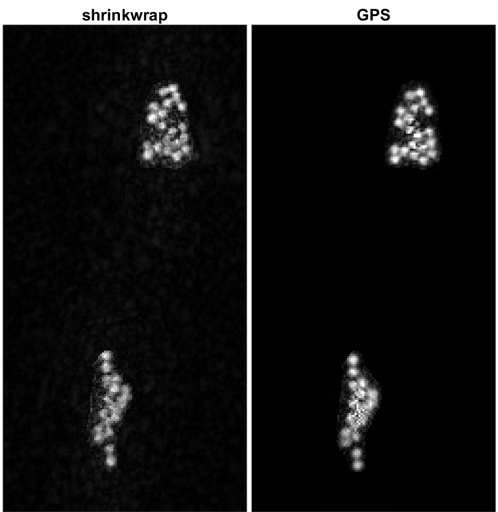
The GPS reconstruction is better than the shrinkwrap code alone.
The GPS Matlab source codes are freely available at our website.
Please click
here to download the Matlab
code and Code Instruction.
Alternative download link: zenodo link.