(with Multislice Simulation and Experimental Data, and MATLAB Source Codes)
Dislocations and defects strongly influence many of the properties of materials, ranging from the strength of metals and alloys to the efficiency of light-emitting diodes and laser diodes [1-3]. Presently several experimental methods can be used to visualize dislocations. Transmission electron microscopy (TEM) has long been used to image dislocations in materials [4-8]. A TEM image, however, represents a 2D projection of a 3D object. Using weak-beam dark-field [9] and scanning TEM (STEM) [10], electron tomography has been used to image 3D dislocations at a resolution of ~5 nm [11]. Recently, we have achieved 3D imaging of dislocations in a platinum (Pt) nanoparticle at atomic resolution using electron tomography [12]. To facilitate those who may be interested in this work, here we provide multislice simulation and experimental data, and MATLAB source codes for observing 3D dislocations in the Pt nanoparticle at atomic resolution.
I. Multislice Simulation Data with EST Reconstructions and 3D Fourier Filtering :
We first performed multislice STEM calculations of a decahedral Pt nanoparticle.
The Pt particle with a size of 7.3nm × 7.0nm × 4.5nm includes edge and screw dislocations. Figures 1a and b show two 2.6 Å thick central slices of the simulated nanoparticle in the XY and ZX planes, where the Z-axis is the beam direction. A zoomed view of an edge dislocation is shown in Fig. 1c. Using multislice STEM calculations [13], a tilt series of 63 projections with a tilt range of ±72.6° and equal slope increments was obtained [12,14-18]. To simulate experimental conditions, the tilt angles were continuously shifted from 0° to 0.5° over the process of the tilt series. Two levels of Poisson noise were added to the projections of the tilt series with a total electron dose of 2.52×10⁵ and 5.67×10⁴ e/Å2, corresponding to Rnoise of 10% and 20%, respectively, defined as
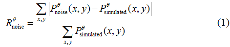
where Pθsimulate (x,y)is the projection calculated from multislice STEM simulations at angle θ, and Pθnoise(x,y) is the same projection with Poisson noise added. After computing for each projection, we calculated Rnoise by averaging Rθnoise for all the projections. The two tilt series were aligned and reconstructed by the center of mass (CM) and EST methods [12,14-18]. Figures 1d-f show the corresponding 2.6 Å thick slices and the edge dislocation reconstructed from 63 multislice STEM projections with Rnoise = 10%. After applying a 3D Fourier filter to the raw reconstruction, we obtained a 3D structure of the simulated Pt nanoparticle in which the atoms are resolved and the edge dislocation is clearly visible (Figs. 1g-i). We also applied the same 3D Fourier filter to the 3D reconstruction with Rnoise = 20% (Figs. 1j-l). Figures 1m-o show the corresponding 2.6 Å thick slices in which the edge dislocation is still visible. In our numerical simulations, we have also found that 3D Fourier filtering is more accurate than the 2D case (Fig. 2).
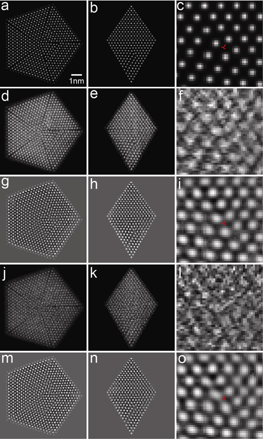
Figure 1. Multislice STEM data with EST reconstructions and 3D Fourier filtering.a and b, Two 2.6 Å thick central slices of the Coulomb potential of a simulated Pt nanoparticle in the XY and ZX planes, where the Z-axis is the beam direction. c, Zoomed view of an edge dislocation in a 2.6 Å thick slice, obtained after a -90° rotation of the nanoparticle around the Y-axis and another -35.3° rotation around the Z axis. d, e and f, The corresponding 2.6 Å thick slices and the edge dislocation reconstructed from 63 multislice STEM projections with Rnoise = 10%. g, h and i,, The corresponding 2.6 Å thick slices and the edge dislocation with Rnoise = 10%, after applying a 3D Fourier filter with an optimized threshold of 5% of the highest intensity {111} Bragg peak. Compared to the threshold (10%) used for the experimental Pt nanoparticle, a smaller threshold (5%) here is because cross-streak noise in this reconstruction is lower than that in the experimental data. The clear boundary of the reconstructed nanoparticle is due to the multiplication of the filtered structure with a 3D shape obtained from the EST reconstruction. j, k and l, The corresponding 2.6 Å thick slices and the edge dislocation from the raw reconstruction with Rnoise = 20%. m, n and o, The corresponding 2.6 Å thick slices and the edge dislocation with Rnoise = 20% after applying a 3D Fourier filter with a threshold of 5%. With Fourier filtering, the 3D core structure of the edge dislocation is observed at atomic resolution (i and o) and consistent with the model (c).
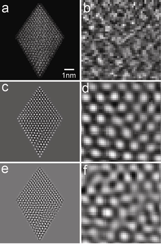
Figure 2. 3D Fourier filtering is more accurate than the 2D case. a and b, A 2.6 Å thick slice and an enlarged view of an edge dislocation, obtained from a 3D reconstruction with Rnoise = 20% (the same as Figs. 1k and l). c and d, The corresponding 2.6 Å thick slices and zoomed view of the edge dislocation with 3D Fourier filtering (the same as Figs. 1n and o). e and f, The corresponding 2.6 Å thick slices and zoomed view of the edge dislocation with 2D Fourier filtering, in which artifacts are clearly visible.
1) Click
here to download the 3D model of the Pt nanoparticle.
2) Click
here to download the 3D EST reconstruction with Rnoise = 10%.
3) Click
here to download the 3D EST reconstruction with Rnoise = 20%.
4) Click
here to download the MATLAB source code for applying 3D Fourier filtering to the EST reconstructions with Rnoise = 10% and displaying the edge dislocation.
5) Click
here to download the MATLAB source code for applying 3D Fourier filtering to the EST reconstructions with Rnoise = 20% and displaying the edge dislocation.
II.Experimental Data with EST Reconstructions, 3D Fourier, and 3D Werner Filtering
The electron tomography experiment was conducted using a FEI Titan 80-300 microscope (energy: 200 keV; spherical aberration: 1.2mm; illumination semi-angle: 10.7 mrad). The scattered electrons were captured by a Fischione 3000 high-angle annular dark-field (HAADF) detector with angles between 35.2 mrad and 212.3 mrad relative to the optical axis. HAADF angles were used to reduce the nonlinear intensities and the diffraction contrast in the images. Using a low-exposure acquisition scheme [12,18], a tomographic tilt series of 104 projections with equal-slope increments and a tilt range of ±72.6° was acquired from a Pt nanoparticle. After performing background subtraction and CM alignment, the tilt series was reconstructed by the EST method [12,14-18]. To enhance the single to noise ratio in the reconstruction, we applied 3D Fourier filtering to the EST reconstruction based on the following procedure [12]. First, the 3D Fourier transform of the raw reconstruction of the Pt nanoparticle consists of two sets of lattice planes {111} and {200}. The intensities of the {111} peaks were estimated to be several times higher than those of the {200} peaks. We calculated the average radial distance (d) between the {111} and {200} peaks. Two radii were then determined by Rin = R111 − d and Rout = R200 + d, where R111 and R200 are the average radial distance for the {111} and {200} peaks, respectively. By keeping those voxels in the 3D Fourier transform with their radii between Rinand Rout, and setting other voxels to zero, we obtained a two-shell volume including all the measurable 3D Bragg peaks.
Next, we implemented a method to further reduce noise among the Bragg peaks within the two-shell volume. We chose the most intense {111} Bragg peak as a reference peak and calculated thresholds based on the reference peak. We scanned the thresholds from 1% to 20% of the reference peak in steps of 1%. For each threshold, we set voxels with values larger than the threshold to one and other voxels to zero, and obtained a 3D mask. The 3D mask was convolved with a three-voxel-diameter sphere to compute a new 3D mask, where the convolution process was to retain the 3D distribution of each Bragg peak. By multiplying the new 3D mask with the Fourier transform of the raw reconstruction, we obtained a new 3D Fourier transform. By monitoring the change in the noise among the Bragg peaks, we found that a threshold with ~10% of the reference peak is large enough to remove noise among the 3D Bragg peaks, while retaining all the measurable {111} and {200} peaks and the 3D distribution around each peak. The optimized threshold of ~10% of the reference peak obtained here may vary for different samples.
Finally, by applying the inverse Fourier transform to the filtered pattern and multiplying it by a 3D shape (that is, a tight support) obtained from the EST reconstruction, we obtained the 3D structure of the Pt nanoparticle. To visualize a screw dislocation, a 5.3-Å-thick slice (two atomic layers) in the (111) plane was selected from the Pt structure and then tilted to the [011] direction. Figure 3a and b show surface renderings of an enlarged view of the slice, corresponding to a threshold of 7% and 10%, respectively. The atoms indicated by green dots are in the top layer and those indicated by red dots are in the bottom layer. The zigzag pattern, a characteristic feature of a screw dislocation, is visible in both images and the Burgers vector of the screw dislocation was determined to be ½[011] . To further verify the 3D Fourier filtering method, we performed a comparison with a 3D Wiener filter using the same experimental data. The Wiener filter is well established for reducing the noise in a signal [19], and it is used to TEM images [20]. 3D Wiener filtering was applied to the EST reconstruction with varying λ where λ is a parameter that controls the filtering strength (larger values of λ give stronger filtering). Figure 3c and d show the same screw dislocation in the Pt nanoparticle with λ = 2 and 3, respectively, which agree with the 3D Fourier filtering results (Figs. 3a and b).
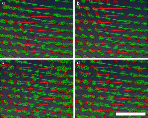
Figure 3. 3D atomic-resolution imaging of a screw dislocation in a Pt nanoparticle using experimental data. Surface renderings of an enlarged view of a 5.3-Å-thick slice (two atomic layers) in the (111) plane, tilted to the [011] direction to visualize the zigzag pattern, a characteristic feature of a screw dislocation. a and b, The 3D core structure of the screw dislocation obtained by applying 3D Fourier filtering to the EST reconstruction with threshold = 7% and 10%, respectively. c and d, The 3D core structure of the screw dislocation obtained by applying 3D Wiener filtering to the EST reconstruction with λ= 2 and 3, respectively. Note that the images shown here have a larger field of view and are also slightly tilted relative to Figs. 3c and d in ref. 12. Scale bar: 1 nm.
1) Click
here to download the 3D EST reconstruction of the Pt nanoparticle from an experimental tilt series.
2) Click
here to download the MATLAB source code for applying 3D Fourier filtering to the EST reconstruction with threshold = 7% and displaying the screw dislocation (Amira script for better visualization).
3) Click
here to download the MATLAB source code for applying 3D Fourier filtering to the EST reconstruction with threshold = 10% and displaying the screw dislocation (Amira script for better visualization).
4) Click
here to download the MATLAB source code for applying 3D Wiener filtering to the EST reconstruction with λ = 2 and displaying the screw dislocation (Amira script for better visualization).
5) Click
here to download the MATLAB source code for applying 3D Wiener filtering to the EST reconstruction with λ = 3 and displaying the screw dislocation (Amira script for better visualization).
This document was prepared by Jianwei Miao and Chien-Chun Chen in the Department of Physics & Astronomy and California NanoSystems Institute, University of California, Los Angeles, California, 90095, USA. Email: miao@physics.ucla.edu.
References:
1.Hull, D. & Bacon, D. J. Introduction to dislocations 5th ed. (Butterworth-Heinemann, 2011).
2.Smith, W. F. & Hashemi, J. Foundations of Materials Science and Engineering 4th ed. (McGraw-Hill Science, 2005).
3.Nakamura, S. The Roles of Structural Imperfections in InGaN-Based Blue Light-Emitting Diodes and Laser Diodes. Science 281, 956-961 (1998).
4.Hirsch, P. B., Horne, R. W. & Whelan, M. J. LXVIII. Direct observations of the arrangement and motion of dislocations in aluminium. Philos. Mag. 1, 677-684 (1956).
5.Bollmann, W. Interference Effects in the Electron Microscopy of Thin Crystal Foils. Phys. Rev.103 , 1588–1589 (1956).
6.Menter, J. W. The Direct Study by Electron Microscopy of Crystal Lattices and their Imperfections.Proc. R. Soc. Lond.A 236 , 119-135 (1956).
7.Howie, A. & Whelan, M. J. Diffraction Contrast of Electron Microscope Images of Crystal Lattice Defects. III. Results and Experimental Confirmation of the Dynamical Theory of Dislocation Image Contrast.Proc. R. Soc. Lond.A 267 , 206-230 (1962).
8.Hirsch, P. B., Cockayne, D. J. H., Spence, J. C. H. & Whelan, M. J. 50 Years of TEM of dislocations: Past, Present and Future.Philos. Mag. 86, 4519–28 (2006).
9.Cockayne, D. J. H., Ray, I. L. F. & Whelan, M. J. Investigations of dislocation strain fields using weak beams. Philos. Mag. 20, 1265-1270 (1969).
10.Pennycook, S. J. & Nellist, P. D. Scanning Transmission Electron Microscopy: Imaging and Analysis 1st ed. (Springer, 2011).
11.Barnard, J. S., Sharp, J., Tong, J. R. & Midgley, P. A. High-Resolution Three-Dimensional Imaging of Dislocations. Science 313, 319 (2006).
12.Chen, C.-C., Zhu, C., White, E. R., Chiu, C.-Y., Scott, M. C., Regan, B. C., Marks, L. D., Huang, Y. & Miao, J. Three-dimensional imaging of dislocations in a nanoparticle at atomic resolution. Nature 496, 74-77 (2013).
13.people.ccmr.cornell.edu/~kirkland.
14.Miao, J., Föster, F. & Levi, O. Equally sloped tomography with oversampling reconstruction. Phys. Rev. B 72, 052103 (2005).
15.Lee, E. et al. Radiation dose reduction and image enhancement in biological imaging through equally sloped tomography. J. Struct. Biol. 164, 221–227 (2008).
16.Fahimian, B. P., Mao, Y., Cloetens, P., & Miao, J. Low dose X-ray phase-contrast and absorption CT using equally-sloped tomography. Phys. Med. Biol. 55, 5383-5400 (2010).
17.Zhao, Y. et al. High resolution, low dose phase contrast x-ray tomography for 3D diagnosis of human breast cancers. Proc. Natl. Acad. Sci. USA 109, 18290-18294 (2012).
18.Scott, M. C., Chen, C.-C., Mecklenburg, M., Zhu, C., Xu, R., Ercius, P., Dahmen, U., Regan, B. C. & Miao, J. Electron tomography at 2.4 Å resolution. Nature 483, 444–447 (2012).
19.Brown, R. G. & Hwang, P. Y. C. Introduction to Random Signals and Applied Kalman Filtering 3rd ed. (New York: John Wiley & Sons, 1996).
20.Marks, L. D. Wiener-filter enhancement of noisy HREM images. Ultramicroscopy 62, 43-52 (1996).