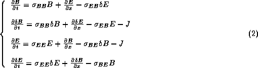
The system to discretize
is replaced by the extended system
where ![]() ,
, ![]() ,
, ![]() , and
, and ![]() are four
free additional parameters which will be used in the discretized
approximation, either to model a physical effect (some dispersion with
are four
free additional parameters which will be used in the discretized
approximation, either to model a physical effect (some dispersion with
![]() for example), either to adjust some numerical corrections or to
model a specific boundary condition. The variables E and
for example), either to adjust some numerical corrections or to
model a specific boundary condition. The variables E and ![]() are
defined by
are
defined by ![]() where
where ![]() and
and ![]() are the components propagating respectively forward and backward
along the axis, with identical definitions for B.
are the components propagating respectively forward and backward
along the axis, with identical definitions for B.
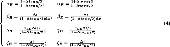
The discretized system takes the form
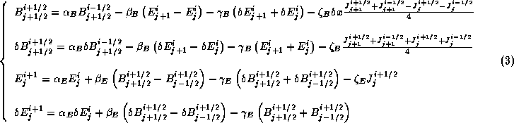
with
In practice, a numerical correction of the form ![]() .
. ![]() must be added to the first equation of the set
(2)in order to satisfy the static limit
must be added to the first equation of the set
(2)in order to satisfy the static limit ![]() in vacuum.
in vacuum.
For ![]()
![]() , the system
(2) reduces to
(1) because, in vacuum, we have
, the system
(2) reduces to
(1) because, in vacuum, we have ![]() and
and ![]() :
:
For ![]() at a boundary, the system reduces
to the usual one-dimensional Sommerfeld outgoing-wave boundary condition and
is extended to the second order approximation of the Engquist and Majda
outgoing-wave boundary condition in higher dimension.
at a boundary, the system reduces
to the usual one-dimensional Sommerfeld outgoing-wave boundary condition and
is extended to the second order approximation of the Engquist and Majda
outgoing-wave boundary condition in higher dimension.
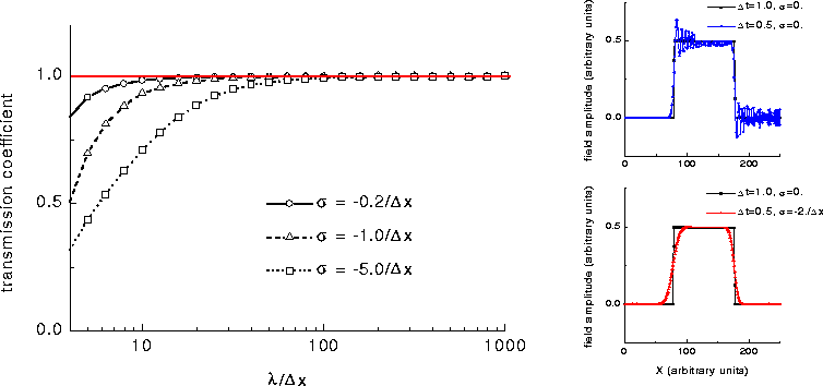
Figure 1: ![]() (when nonequal to zero) has an effect when using the
discretized form of the equations. On the left, it is shown that the short
wavelength waves (
(when nonequal to zero) has an effect when using the
discretized form of the equations. On the left, it is shown that the short
wavelength waves ( ![]() is the mesh size) are damped when
is the mesh size) are damped when ![]() .
A benefit of this damping is a tunable reduction of numerical noise, has shown
on the right where the response of the system to a heavyside signal is
displayed for
.
A benefit of this damping is a tunable reduction of numerical noise, has shown
on the right where the response of the system to a heavyside signal is
displayed for ![]() (top) and for
(top) and for ![]() (bottom).
(bottom).